How to Calculate Uncertainty in Physics (Step-by-Step)

I wrote this article for students who are starting out with A-level or introductory physics.

For this reason, while explaining how to calculate uncertainty, I’ll consider only the uncertainty arising due to the least count of the measuring instrument. This is the approach most introductory physics textbooks follow.

Other sources of uncertainty are deliberately excluded to keep things simple for beginners.

For a deeper explanation that includes every source of uncertainty, you may want to check the UKAS guide.

While calculating uncertainty, you will usually come across three main situations.

Sometimes you only have a single measurement to work with. Other times, you collect multiple readings of the same quantity and calculate the final uncertainty.

And in some experiments, such as repeated motions or a stack of identical objects. Here, uncertainty is handled in a slightly different way to improve accuracy. Let’s discuss all of these situations one by one.

Steps to Calculate Uncertainty for a Single Value of Measurand

For introductory or A-level physics, follow these steps to calculate uncertainty when you have a single value of a measurand (required quantity).

1) Formula Used to Calculate the Desired Quantity

If you want to find a quantity that involves a formula, the first step is to write down that formula.

Doing this shows which quantities must be measured to find the value of the required quantity (measurand). It also helps you understand where uncertainty comes from in the final result.

For example, if you want to find the Gravitational force, the formula would be

F=G\;\frac{m_1\;m_2}{r^2}

This means that to find the total uncertainty in gravitational force, you must combine the uncertainties in the gravitational constant (G), the masses (m₁ and m₂), and the square of the distance between them (r²).

To combine all these uncertainties, there are certain rules that are explained in step 6.

If the procedure involves the direct measurement of the required quantity, you can skip step 1 and start from step 2.

2) Record the Value of Measured Quantities and Measurand

Once the formula is clear, the next step is to measure all quantities needed to calculate the desired quantity.

Continuing with the gravitational force example, you would measure the masses m₁ and m₂, and the distance r between them. Let’s say their values are

m_1=54.4\;\mathrm{kg}

m_1=37.8\;\mathrm{kg}

r\;=\;93.6\;\mathrm m

For convenience, take the value of the gravitational constant from a trusted textbook like Physics Volume 1, 5th edition by HRK. The value in this book is 6.673 x 10^-11 N m²/kg².

To calculate the value of the measurand (gravitational force), we have

F=G\;\frac{m_1\;m_2}{r^2}

=\;6.673\;x\;10^{-11}\;\frac{\;(54.4)\;(37.8)}{{(93.6)}^2}\;

= 6.673 x 10^-11 x 2056.32 / 8760.96

= 1.37218234 x 10^-7 / 8760.96

F=1.57\;x\;10^{-11}\;\mathrm N

This is the gravitational force between two objects.

As we only round off in the final step to avoid excessive rounding error, that’s why I underlined the last significant digit in each calculation. If you’re wondering how I rounded the final result, you can check the detailed article on significant figures.

3) Determine the Absolute Uncertainty of Each Measurement

While recording the measurement, you also need to write down the uncertainty that arises during each measurement.

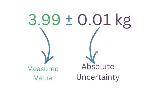
The uncertainty that you write with the measured value using the number and unit is known as absolute uncertainty. For example, 3.99 ± 0.01 kg

Image showing how the absolute uncertainty looks and how you write it with measured value

Rules For Writing Uncertainty:

When you write uncertainty with the measured value, there are some special rules to follow

1) We usually report uncertainty with one significant figure to avoid implying false precision.

However, you may keep two significant figures in some cases to reduce excessive rounding.

2) The measured value and its uncertainty must have the same precision, meaning they align to the same decimal place.

If the uncertainty is large, the measured value should be rounded so that unnecessary extra digits are removed. If the uncertainty is small, you may need to include extra digits in the measured value to match its precision.

According to this rule, if the uncertainty is half the smallest division, we need to estimate one extra digit between the scale marks to match the precision of both the measured value and uncertainty.

For example, a thermometer with a smallest division of 1 K has an uncertainty of ± 0.5 K.

By estimating between the marks, we can record a reading like 23.4 K, where the first uncertain digit is in the tenths place.

According to these rules, we should round off the uncertainty or measured value where there are extra digits. But take this step only at the end to avoid excessive rounding errors.

Whether the uncertainty is half or full smallest division depends on how many judgments you make during the measurement.

Uncertainty in a Measurement (involves two judgements):

If a measurement requires two estimates (judgements), we usually take the uncertainty as the full smallest division (the instrument’s least count).

For example, when measuring length with a ruler, you must align one end of the object with the zero mark and read the position of the other end. Since both ends involve an estimate, the combined effect leads to the final uncertainty, half of the smallest division from each.

Uncertainty in a reading (involves one reading):

If a measurement requires only one estimate, the uncertainty is taken as half of the smallest division. For instance, in a thermometer, the zero reference is already fixed. So, you only estimate one position (the liquid level), and the uncertainty is half of the smallest division.

Uncertainty in Digital Meters:

Digital readings either have an uncertainty specified by the manufacturer or (if not given) an uncertainty taken as ±1 in the last displayed digit.

For example, if the digital reading is 3.2 kg, the uncertainty in the last displayed digit is ± 0.1 kg.

Suppose you measure the masses m₁ and m₂ with a digital scale (least count 0.1 kg) and the distance between the objects with a ruler (least count 0.1 m).

So the uncertainty in the value of masses m1 and m2 will be ± 0.1 kg, and the uncertainty in the distance between them is ± 0.1 m.

Also, the uncertainty in the value of the gravitational constant is taken from the textbook (Physics Volume 1, 5th Edition by HRK), which is ± 0.010 x 10^-11 N m²/kg².

4) Express Measurements with Their Absolute Uncertainties

We have found the measurements and uncertainties of each value involved; let’s write them together as convention.

m₁ = 54.4 ± 0.1 kg

m₂ = 37.8 ± 0.1 kg

r = 93.6 ± 0.1 m

G = 6.673 x 10^-11 ± 0.010 x 10^-11 N m²/kg².

5) Find the Relative or Percentage Uncertainty (if required)

We add relative (or percentage) uncertainty whenever we multiply or divide quantities in a formula.

The quantities in formual that involve multiplication or division, find their relative and percentage uncertainties.

The formulas to calculate relative and percentage uncertainties are

\[Relative\;or\;Fractional\;uncertainty=\frac{Absolute\;uncertainty}{Measured\;value}\]

\[Percent\;uncertainty=Relative\;uncertainty\;\times\;100\]

\[Percent\;uncertainty=\frac{Absolute\;uncertainty}{Measured\;value}\times100\]

In the gravitational force formula, G, m₁, and m₂ involve multiplication and division by r². So, we need to calculate the relative and percentage uncertainty of all these quantities.

For m₁,

Relative uncertainty = Δm₁ / m₁ = 0.1 / 54.4 = 0.0018

Percent uncertainty = Δm₁ / m₁ x 100 = 0.0018 x 100 = 0.18%

For m₂,

Δm₂ / m₂ = 0.1 / 37.8 = 0.0026

Δm₂ / m₂ x 100 = 0.0026 x 100 = 0.26%

For r,

Δr / r = 0.1 / 93.6 = 0.0011

Δr / r x 100 = 0.0011 x 100 = 0.11%

For G,

ΔG / G = 0.010 x 10^-11 / 6.673 x 10^-11 = 0.0015

ΔG / G x 100 = 0.0015 x 100 = 0.15%

Avoid rounding off during intermediate calculations. Keep extra digits (guard digits) so rounding errors don’t accumulate.

After combining all uncertainties, round the final value of uncertainty to one significant figure (or two, if needed).

6) Uncertainty Propagation to Obtain the Final Uncertainty (Combining Individual Uncertainties)

Uncertainty propagation is the process of combining the uncertainties of all measured values according to the formula used to calculate the desired quantity.

In the continuing example of gravitational force, you multiply G, m₁, and m₂ and divide them by r².

Multiplication Uncertainty Rule

Whenever two or more quantities are multiplied, their relative uncertainties are added.

While calculating the gravitational force, G, m₁, and m₂ are multiplied, so their relative uncertainties would be added. So, the multiplication uncertainty formula is

\frac{\;\Delta Q}Q=\overset n{\underset{i=1}{\sum\;}}\frac{\Delta X_i}{X_i}

Where ΔQ and ΔX_i are the uncertainties in the values Q and X_i (i can be any positive integer).

\frac{\mathit\Delta\mathit Q}{\mathit Q}\;=\;\frac{\mathit\Delta\mathit G}{\mathit G}+\frac{\Delta m_1}{m_1}+\frac{\Delta m_2}{m_2}

\[=0.0015+0.0018+0.0026\]

\[=0.0059\]

Power Factor Uncertainty Rule

When a quantity is raised to a power n, like Q = Aⁿ, it is equivalent to multiplying the same quantity by itself n times.

Therefore, the relative uncertainty is added as many times as the power. The formula, when the power factor is involved, is

\frac{\Delta P}P=\frac{\Delta A}A+\frac{\Delta A}A+\frac{\Delta A}A+\dots\dots.\;(n\;times)

\frac{\Delta P}P=n\times\frac{\Delta A}A

Where ΔP and ΔA are uncertainties in values P and A.

Division Uncertainty Rule

Similar to multiplication, when two or more quantities are divided, their relative uncertainties are added. So the formula for this would be the same as that of mutliplication uncertainty formula, i.e.

\frac{\;\Delta Q}Q=\overset n{\underset{i=1}{\sum\;}}\frac{\Delta X_i}{X_i}

Where ΔQ and ΔX_i are the uncertainties in the values Q and X_i (i can be any positive integer).

According to the gravitational force formula, the quantities G, m₁, and m₂ are divided by r². It means that ΔQ / Q and Δr² / r² are added to get the final relative uncertainty of the gravitational force.

\frac{\Delta F}F=\frac{\Delta G}G+\;\frac{\Delta m_1}{m_1}+\frac{\Delta m_2}{m_2}+2\times\frac{\Delta r}r

=\frac{\Delta Q}Q+2\times\frac{\Delta r}r

= 0.0059 + 0.0022

\frac{\Delta F}F=0.0081

The value obtained represents the relative uncertainty of the gravitational force.

If you like calculations using percentage uncertainties, you can follow the same method with percentages instead. Both methods are equivalent, so the final result will remain the same.

Addition / Subtraction Uncertainty Rule

Whenever two or more quantities are added or subtracted, their absolute uncertainties are added.

For example, we have

L_1=27.3\pm0.1\;\mathrm{cm}

L_2=35.2\pm0.1\;\mathrm{cm}

L_2-L_1=7.9\pm0.2\;\mathrm{cm}

Although we don’t need this rule in our example, it is helpful when you’re dealing with addition or subtraction.

7) Express the Final Result with Uncertainty Using Proper Significant Figures

To express the uncertainty with the final result, we need to convert the relative uncertainty into absolute uncertainty by carrying out one more step in the calculation.

\frac{\Delta F}F=0.0081

F\times\frac{\Delta F}F=0.0081\times F

\Delta F=0.0081\times1.57\times10^{-11}\;\mathrm N

\Delta F=1.2717\times10^{-13}\;\mathrm N

According to the rules, round the uncertainty to one significant digit, and make the measured value match this precision. So, the final result with uncertainty, we can write it as

F = 157 x 10^-13 ± 1 x 10^-13 N
Or
F = 1.57 x 10^-11 ± 0.01 x 10^-11 N

Both are correct. It’s best to express the final result in scientific notation.

Steps to Calculate Uncertainty from Repeated Values of Measurand

If you’re asked to repeat the same measurement, and calculate the uncertainty due to all these repeated values. The process would be different from single-value measurement.

One method is take the difference between the maximum and minimum measured values in the repeated measurements and then divide it by 2. The answer gives the uncertainty in repeated values.

Uncertainty=\frac{(Maximum\;value\;-\;Minimum\;value)}2

But there is one more detailed method in the introductory physics books that gives better approximations.

1) Record the multiple measurements of the measurand

Begin by measuring the quantity you are interested in (the measurand) several times.

The more measurements you take, the more reliable your estimate of the uncertainty will be.

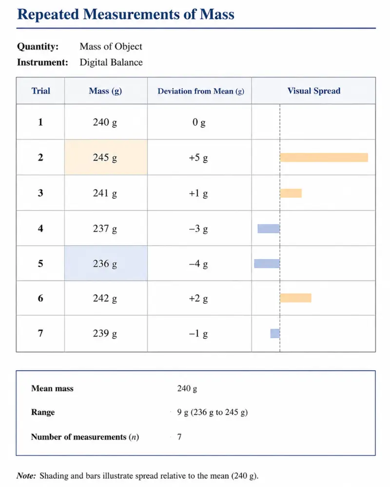
Let’s say you want to measure the mass of your book with a digital balance having the least count of 1 g. You repeat the same experiment 7 times and get the values

240 g, 245 g, 241 g, 237 g, 236 g, 242 g, 239 g

2) Take the average of these measurements

Add up all the measured values and divide by the total number of measurements. This gives the mean (or average) value, which serves as the best estimate of the measurand.

Average = 240 + 245 + 241 + 237 + 236 + 242 + 239 / 7

= 1680 / 7

Average = 240 g

3) Calculate the deviation of each measurement from the average value

Subtract the mean value from each measurement. This shows how far each individual measurement is from the average.

0 g, 5 g, 1 g, -3 g, -4 g, 2 g, -1 g

4) Take the absolute value of the deviation of each measurement

Since we are interested in the size of the deviation regardless of its direction (above or below the mean), take the absolute value of each deviation.

This ensures that all deviations contribute positively to the uncertainty. So, the final deviation of each measure with absolute value is

0 g, 5 g, 1 g, 3 g, 4 g, 2 g, 1 g

5) Calculate the mean of deviation (This is your uncertainty)

Add up all the absolute deviations and divide by the total number of measurements. This gives the mean absolute deviation, which is taken as the uncertainty of the measured quantity.

= 0 + 5 + 1 + 3 + 4 + 2 + 1 / 7

= 16 / 7

Mean of deviation = 2.2857 g

According to the uncertainty rule, the measured value and uncertainty should have the same precision. Additionally, always round the uncertainty to 1 sig fig.

So, the final uncertainty becomes 2 g.

If we express it with the best estimate, the answer is
240 ± 2 g.

Steps to Calculate Uncertainty in the Timing Experiment

In experiments like a simple pendulum, where you determine an object’s time period from its repeated motion, follow these steps to calculate uncertainty:

1) Measure the Total Time Taken for Multiple Vibrations

Let’s take the example of a simple pendulum. A simple pendulum is a weight hanging on a string that swings freely to and fro. The pendulum takes 20 vibrations, you record the total time with a stopwatch as 34.5 s.

The smallest time interval the stopwatch can measure is 0.1 s.

2) Determine the Uncertainty in the Total Measured Time

Since you make two timing judgments. One when starting the stopwatch and one when stopping it.

The uncertainties from both contribute to the total timing uncertainty. As the reaction-time uncertainty is ±0.05 s for each judgement, the total uncertainty becomes ±0.1 s.

3) Calculate the Time Period

The time period is the time needed to complete one full vibration. To calculate the time period, we divide the total time by the total number of vibrations. The value we have
T = 34.5 / 20 = 1.725 s

Based on significant figure division rules, the final answer should have the same number of significant digits as the value with the fewest significant digits. Hence, the T = 1.72 s

4) Calculate the Uncertainty in the Time Period

To calculate the total uncertainty in the time period, divide the total uncertainty by the total number of vibrations. It would give you uncertainty in one complete vibration.

ΔT = 0.1 / 20 = 0.005 s

This is the absolute uncertainty in the time period.

5) Express the Uncertainty with the Time period

The final step is express the uncertainty with the time period. This step is the same as the step in previous methods. So, we have

T = 1.72 ± 0.005 s

According to the uncertainty, the measured value and the uncertainty should be of the same precision. So, for this special case, we have to take the final value as

T = 1.725 ± 0.005 s

These steps don’t apply only to timing experiments. The same idea works whenever you measure a group of identical items. Instead of measuring one tiny item, measure a stack (e.g., coins, CDs, sheets, wires) and then calculate the value for one. It reduces the uncertainty of measurement.